Scientific journal
European Journal of Natural History
ISSN 2073-4972
ИФ РИНЦ = 0.204
THEORETICAL STUDIES OF STUDENT BEHAVIOR IN THE PROCESS OF ACQUIRING KNOWLEDGE
Introduction
Currently, probabilistic-statistical methods are widely used in conducting psychological and pedagogical research, which include the classical or mass probabilistic-statistical method (MPS-method) and the non-classical or individual probabilistic-statistical method (IPS-method). The MPS-method is used to analyze the behavior of a large number of objects or events, because it is in this case that statistical patterns become apparent [1, 2]. The IPS-method is used to analyze the behavior of individual objects, which internally have a random character of behavior. Such objects include quantum objects (electrons, atoms, etc.) and a person in the process of activity, for example, a student in the process of acquiring knowledge [3, 4].
In the process of acquiring knowledge (assimilation of information), the student moves in the information space, which is a set of results of the semantic activity of mankind. Academic disciplines contain information blocks arranged in a strict logical sequence. This means that there are certain directions in the information space, along which students move. In computer science, information is usually measured in bits, and in pedagogy, when measuring students’ knowledge, in points. There is a certain relationship between bits of information and scores, namely, the maximum score of the selected measurement scale corresponds to the amount of information contained in the academic discipline.
In accordance with the IPS-method, the student is identified by a differential distribution function (probability density), and, consequently, we can only talk about the probability of finding the student in one or another area of the information space [3]. Hereafter, for reasons of brevity, we will call the differential distribution function simply a distribution function. The student’s knowledge is random in nature, since it is a product of his consciousness (the work of the brain), the determinism of which is realized through randomness due to the random nature of the psychosomatic state of a person. These arguments formed the basis for constructing a probabilistic-statistical model of the student, according to which he is identified by the distribution function in the information space.
The purpose of the study is the theoretical substantiation and application of an individual probabilistic-statistical method for analyzing the behavior of a student in the process of acquiring knowledge.
Materials and research methods
The distribution functions that identify the student are solutions of differential equations obtained on the basis of the law of conservation of probability [3]. They are continuity equations that relate the change of probability density per unit of time in the space of coordinates, velocities and accelerations of various orders with the divergence of the probability flux density. These equations have the following form:

..................................................................................... , (1)
where,  ,
,  and
and  are the distribution functions identifying the student in the information space;
  are coordinate, velocity, average velocity, first–order acceleration, average first-order acceleration and average second–order acceleration, respectively; t is time.
This system consists of an infinite number of equations, and the question of which of the above equations to use to find the distribution function depends on the possibility of obtaining data on the average values of velocity and accelerations of various orders.
The first equation from the system of differential equations (1) allows us to explicitly find the distribution function describing the behavior of the student in coordinate space. We will now find a solution to this equation by writing it in the follo wing form:
 . (2)
. (2)
The solution to this equation is the argument function  , namely,
 . (3)
. (3)
This can be verified by substituting (3) into (2). We will find a specific form of distribution function from the analysis of experimental material. To this end, we will use an experimental distribution function that identifies the student, obtained using the IVS method on a twenty-point scale and corresponding to 3 points on a five-point scale [5] (fig. 1).
The experimental distribution function is presented in the form of a histogram, which was obtained by averaging 28 individual distribution functions of students who took the physics exam. It is found that the histogram is well approximated by the distribution function (smooth line) corresponding to the law of normal distribution [6]:
 , (4)
, (4)
where σ is the coordinate; < σ > is mathematical expectation; μ is variance.
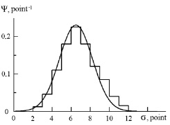
Fig. 1. Distribution function: experimental (histogram); theoretical (smooth line)
When calculating the distribution function according to formula (4), a good approximation of the histogram was obtained at < σ > = 6.5 points and μ = 3 point2. The fact that the distribution function, which identifies the student in the process of acquiring knowledge, corresponds to the law of normal distribution, which describes the random nature of the behavior of a large number of objects, is natural from a mathematical point of view, since mathematics analyzes the general character of the behavior of objects, distracting from their nature. In this case, the random nature of the behavior is common for both a single object (student) and a large number of objects.
Research results and discussion
The joint analysis of equations (3) and (4) makes it possible to explicitly write down the distribution function that identifies the student:
 . (5)
. (5)
Function (5) will be distributed in the information space and in time, without changing its initial form. This means that the variance of the distribution function will remain unchanged, and this contradicts experimental data. We will obtain the information about the nature of changes in the variance of distribution functions over time from the analysis of the evolution of experimental distribution functions. To do this, first consider the evolution of the experimental distribution function obtained using the MPS-method (fig. 2a). This will allow us to find the dependence of the variance on time, and then calculate the theoretical distribution functions that identify the student, in accordance with the IPS-method, using formula (5) and the found dependence of the variance on time. Let’s use a five–point knowledge measurement system, the absolute error in this case is 0.5 points, and the relative error is 10%. The construction of the distribution function will be carried out in terms of one academic discipline per semester in accordance with [5]. Thus, the assessment of a student who received 3 points on the exam should be written taking into account the error in the form of (3.0 ± 0.5) points, where 3 points is the mathematical expectation. This means that the student is identified by a distribution function, the width of which is 1 point, and the height is 1 point – 1. Therefore, after a two-semester year of study, the width of the distribution function will be 2 points, after the second – 4 points, after the third – 6 points, after the fourth – 8 points and after the fifth – 10 points. The average rate of movement of the mathematical expectation is 6 points per year (< >= 6 points /year). The evolution of the distribution function by year is shown in fig. 2.
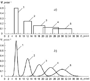
Fig.2. Evolution of distribution functions: a) – obtained by the MPS-method; b) – obtained by the IPS-method; 1, 2, 3, 4, 5 – after the first, second, third, fourth, fifth years of study, respectively
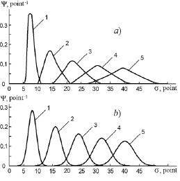
Fig. 3. Evolution of distribution functions: a) – experimental; b) – theoretical; 1, 2, 3, 4, 5 – after 1, 2, 3, 4, 5 years of study, respectively
The distribution functions shown in fig. 2b were calculated using formula (5) using the values of variance obtained by finding the moments of the second-order of rectangular distribution functions (fig. 2a). The analysis of the data presented in fig. 2 shows that the distribution functions obtained using the IPS-method are much more informative than the distribution functions obtained by the traditional MPS-method. Within the framework of a five-point measurement system, due to the large measurement error, it is impossible to obtain experimental distribution functions identifying the student using the IPS-method. This problem is solved when switching to measurement systems with a higher score, for example, to ten-point, twenty-point, hundred-point measurement systems. However, when analyzing the behavior of a large number of students, the distribution functions obtained by the IPS-method can be approximated by rectangular functions that actually coincide in shape with the distribution functions obtained by the MPS-method. This approach to obtaining experimental distribution functions was implemented in [5]. Fig. 3 shows the experimental and theoretical distribution functions.
The experimental distribution function (fig.3a) is taken from [5]. This function was obtained by averaging the individual distribution functions of the student flow (78 people). It can be seen that as we move in the information space, the variance of the distribution functions increases, and the distribution functions themselves overlap, and especially heavily starting from the third year of study. The weak students contributed to the tail part of the distribution function, and the strong students contributed to the head part. By the terms “weak”, “average” and “strong” student we will conditionally understand students who receive an average of three points, four points and five points on exams according to the five-point system, respectively. An analysis of possible theoretical distribution functions has shown that the distribution function identifying the average student (fig. 3b), taking into account the linear dependence of mathematical expectation on time ( , where <
 >= 8 point/year) and variance on time (μ = at, where a = 2 point2 /year), agrees well with the experimental distribution function.
Fig.4 shows the dependences of the theoretical distribution functions on the learning time, describing the behavior of the weak and strong students.
When calculating the distribution functions, linear dependences of mathematical expectation on time were used, which were equal to 6 points/year for the weak student and 10 points/year for the strong student. The time dependence of the variance was assumed to be the same as when calculating the distribution function for the average student.
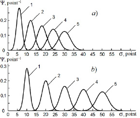
Fig. 4. Evolution of distribution functions: a) – identifying the weak student; b) – identifying the strong student;1, 2, 3, 4, 5 –after 1, 2, 3, 4, 5 years of study, respectively
The analysis of the data shown in fig. 4 showed that the distribution functions identifying the weak student (fig.4a) heavily overlap, especially at senior courses. This means that the weak student, figuratively speaking, seems to be “stuck” in the information space. At the same time, the distribution functions identifying the strong student (fig. 4b) overlap slightly and are significantly ahead of the distribution functions identifying the weak student. This means that co-education of weak students and strong students is not advisable. To ensure optimal conditions for realizing the potential of weak and strong students in the process of obtaining education, it is advisable to switch to a system of step-by-step learning with branching [5].
We will analyze stationary distribution functions – distribution functions that do not depend on time and characterize the stationary state of an object or system. The stationary state corresponds to the condition under which  . Then, in accordance with equation (2), we will have
  . In this case, there are two solutions: the first corresponds to the condition
  , the second – to the condition
  . In the first case, the derivative of the distribution function from the coordinate can be determined by an arbitrary coordinate function, namely,
  , where
  is an arbitrary function. To find the distribution function, we use the following integral transformation
 .
.
In [5], a method for finding the distribution function for this case is considered, based on the use of step functions [7], and the function itself is found, which has the following form
The differential distribution function is obtained in the form of a histogram by averaging the individual distribution functions identifying the students, and then approximated by a smooth line. The distribution function is represented in a dimensionless coordinate system ( ,
,  , where σmax is the maximum value of the scale) and in a twenty-point coordinate system. Using a dimensionless coordinate system is convenient because the distribution function represented in a dimensionless coordinate system has the same appearance in all other coordinate systems. This allows direct translation of the distribution function from one coordinate system to another. Due to the presence of measurement scale boundaries, the distribution function has a “U”-shaped appearance.
Let’s consider the second stationary solution corresponding to the condition  . The solution of this equation is a function independent of the coordinate, namely,
  . This distribution function is the same for both weak and strong students.
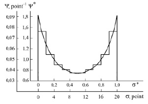
Fig.5. Differential distribution function
This means that the process of transition of the system to a stationary state should last as long as it takes, so that not only strong students could assimilate the material of a particular academic discipline, but also weak students.
Conclusions
1. The solution of the differential equation describing the progress of the student in the information space in the process of obtaining knowledge is obtained. The solution is a distribution function that identifies the student, which in form coincides with the normal distribution.
2. A joint analysis is carried out of the evolution of the experimental student distribution function (obtained by averaging the individual distribution functions of the students of the flow) and the theoretical distribution function identifying the student. It is established that the theoretical distribution function identifying the average student is in good agreement with the experimental distribution function.
3. A comparative analysis of the theoretical distribution functions identifying weak and strong students showed that the distribution functions identifying weak students begin to overlap after the second year of study, and the degree of overlap increases over time. The distribution functions identifying strong students overlap slightly.
4. It is shown that in order to ensure optimal conditions for the realization of the potential opportunities of weak and strong students in the process of obtaining education, it is advisable to use a system of step-by-step learning with branching.
Библиографическая ссылка
Romanov V.P., Shiryaeva N.A. THEORETICAL STUDIES OF STUDENT BEHAVIOR IN THE PROCESS OF ACQUIRING KNOWLEDGE // European Journal of Natural History. 2024. № 5. ;URL: https://world-science.ru/en/article/view?id=34398 (дата обращения: 13.05.2026).
DOI: https://doi.org/10.17513/ejnh.34398

