
Scientific journal
European Journal of Natural History
ISSN 2073-4972
ИФ РИНЦ = 0.204
ECONOMETRIC FORECAST OF THE SHARE PRICE ON THE EXAMPLE OF PJSC “OIL COMPANY “ROSNEFT”

The company’s business planning is based on forecasting the development of its external and internal environment. The identification of objective patterns of development, expressed in the presence of relationships between individual parties of the analyzed phenomena, reflected in the relevant indicators, is a necessary condition for making the right management decisions [1, p. 10], which confirms the relevance of this study. The purpose of this study is an econometric analysis of the factors that affect the share price on the example of the Public Joint Stock Company “Rosneft Oil Company”, and the construction of a model for its forecasting.
The basis of econometric research is the construction of an econometric model, which is based on the assumption that there is a real relationship between the characteristics. An econometric model is an equation or a system of equations where the main quantitative relationships between the analyzed economic processes and objects are described in mathematical form, and insignificant relationships are ignored in the model [2]. In addition to studying the real state of processes or objects, econometric models can predict changes in their state over time. The classification of econometric models is as follows (Fig. 1).
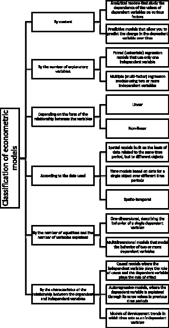
Fig. 1. Classification of econometric models. Source: Compiled by the author
The construction of an econometric model begins with the specification, which consists in determining the economic indicators (features) that should be included in the model, and the type of analytical relationship between these features.
Due to the fact that there is currently a strong volatility in the oil market, the Public Joint Stock Company “Rosneft Oil Company”, which is the leader of the Russian oil industry and the largest public oil and gas corporation in the world, was chosen for this study. The company is included in the list of strategic enterprises of Russia. Its main shareholder (40,4 % of the shares) is ROSNEFTEGAZ JSC, 100 % owned by the state, 19,75 % of the shares belong to BP, 18,93 % – to QH Oil Investments LLC, one share belongs to the state represented by the Federal Agency for State Property Management [3].
To perform the study, the shares of PJSC “NK “Rosneft” were selected as an endogenous variable. One of the main factors influencing the share price is EBITDA – the company’s profit before interest on loans, income tax and depreciation. The share price is also affected by the exchange rate of USD/RUB, Urals and inflation.
EBITDA has the greatest impact on the value of the company, so the share price can directly depend on it.
Inflation in general has a contradictory effect on the stock market, however, the decline in purchasing power is directly the result of rising prices, respectively, the inverse dependence of the share price on inflation can be traced.
Due to the fact that oil prices are presented in dollars, the weakening of the ruble will have a positive impact on the ruble profit of PJSC “NK “Rosneft”, and therefore on the share price.
“Rosneft” is one of the main producers of Urals oil, so it is correct to consider these indicators among the factors influencing the company’s share price.
For the analysis, the quarterly price indicators in rubles for shares for the period from March 2007 to September 2020 were taken. In order to collect a sufficient amount of analyzed data and their comparability, it was decided to consider quarterly values, since EBITDA is published in the consolidated financial statements provided once a quarter.
We will make a correlation matrix to show the relationship between the selected exogenous variables and the endogenous variable and the absence of multicollinearity between the exogenous factors (Table 1).
Table 1
Correlation matrix
|
Share Price (Close) |
EBITDA, million rubles |
URALS |
USD/RUB (Open) |
Inflation rate |
|
|
Share Price (Close) |
1 |
||||
|
EBITDA, million rubles |
0,846811067 |
1 |
|||
|
URALS |
-0,289057752 |
-0,18995049 |
1 |
||
|
USD/RUB (Open) |
0,793520906 |
0,718603868 |
-0,674407691 |
1 |
|
|
Inflation rate |
-0,59474119 |
-0,462877807 |
0,049506197 |
-0,403065513 |
1 |
Source: Compiled by the author.
From this table, it follows that EBITDA, USD/RUB, and the share price have a very strong direct relationship, and, as noted earlier, inflation has a moderate inverse relationship. A weak inverse relationship with the endogenous variable is demonstrated by Urals, but it was decided to leave this factor in the model. It should be noted that EBITDA and USD/RUB strongly correlate with each other, but nevertheless, these are very important factors in the model under study.
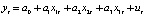
Based on the established economic relationships, the specification of the econometric model can have the form [4]:
yt = a0 + a1x1t + a2x2t + a3x3t + a4x4t + ut,
where yt – the value of the shares of PJSC “NK “Rosneft”
a0 – the risk-free rate of return, unrelated to the studied parameters
x1t – EBITDA amount for the time period t
x2t – URALS for the time period t
x3t – USD/RUB for the time period t
x4t – USD/RUB for the time period t
ut – random residuals.
Thus, the first stage in the formation of the econometric model, consisting in the construction of the specification, was completed.
The second stage is to collect statistics on all the main variables. Since the reports in all companies are published once a year (annual reports) and once a quarter (consolidated reports), in order to collect enough data for analysis, we will take quarterly values for the comparability of all data.
Data on the share prices of “Rosneft”, Urals, USD/RUB, and inflation were downloaded from the Thomson Reuters Eikon terminal, and EBITDA data were calculated manually from the consolidated financial statements [3] using the formula:
EBITDA = Revenue from sales – Costs and expenses + Depreciation and amortization.
Note that until 2011, the Company “Rosneft” reported US GAAP, where data are presented in million us dollars. The US, only since 2012 has moved to IFRS where data is presented in billions [3]. Therefore, for comparability of indicators, it is necessary to translate the data into billion rubles by converting it to the exchange rate. Note that the 2012 financial statements also published data for 2011 [3], which indicates that it is possible to reconcile the translated data at the exchange rate and the data initially available in rubles. Please note that the data do not converge a little, as this is a error of their conversion into another currency manually (so not considered indirect factors that terminal, Thomson Reuters Eikon, and the company PJSC “NK “Rosneft”). This can later become an artificially created structural shift, which will need to be taken into account when building the model.
Thus, the collected statistics are 55 values for the period from March 31, 2007 to September 30, 2020.
For the best analysis of the specification, it is necessary to check the data for outliers and, if any, delete them. Let’s see clearly on the graphs how many outliers are present in the data. (fig. 2, 3).
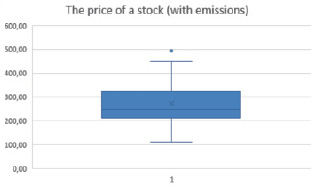
Fig. 2. The presence of emissions in the share price of PJSC “NK “Rosneft” Source: Compiled by the author
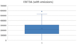
Fig. 3. Presence of emissions in “Rosneft’s” EBITDA” Source: Compiled by the author
This study presents only two graphs out of five, as no outliers were found in the rest.
As can be seen from the figures, the emissions are present in the “Share Price” and “EBITDA” factors, but it should be noted that the emissions correspond to one point in time, respectively, it is enough to remove the emissions from only one factor.
For further research, you need to remove the outliers. Outliers are elements of a variation series that do not belong to a segment.
[x0,25 – 1,5*IQR, x0,75 + 1,5*IQR].
Next, we calculate the boundaries of this segment using such indicators as:
1) The first (Q1 or x0,25) and third (Q3 or x0,75) quartiles
2) Interquartile range (IQR)
Item 1. The first and third quartiles (for the share price) are calculated using the following formulas:
Q1 = КВАРТИЛЬ. ВКЛ (B2: B56; 1)
Q3 = КВАРТИЛЬ. ВКЛ (B2: B56; 3)
Item 2. The interquartile range is found by the following formula:
IQR = Q3 – Q1
After obtaining the values of the above indicators, we determine the left end of the interval (Q1 – 1,5*IQR) and the right end of the interval (Q3 + 1,5*IQR).
Thus, after performing the necessary calculations, we will form a table with all the indicators found (Table 2).
Table 2
Indicators for the removal of emissions
|
Share Price |
EBITDA |
|
|
Q1 |
213,835 |
136500 |
|
Q3 |
320,975 |
307500 |
|
IQR= |
107,14 |
171000 |
|
[Q1-1,5IQR;Q3+1,5IQR] |
||
|
left end of the interval |
53,125 |
-120000 |
|
right end of the interval |
481,685 |
564000 |
Source: Compiled by the author.
Using the obtained data, you need to remove outliers using the Filter tool. After that, the graphs for the data under consideration will look like this (Fig. 4, 5).
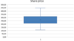
Fig. 4. No emissions in the share price of PJSC “NK “Rosneft” Source: Compiled by the author
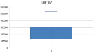
Fig. 5. No emissions in “Rosneft’s” EBITDA Source: Compiled by the author
Thus, by removing outliers from the sample, we improved the quality of the specification of the proposed model.
For further analysis of the specification, we will divide the sample into a training and a control sample, since all analysis will be performed only on the training sample, and the control sample is necessary at the last stage of building the model to check its adequacy.
As a rule, the control sample is taken in the amount of 5-10 % of the total sample. Based on our volume of statistics, we will take a control sample of 4 values, namely (Table 3):
Table 3
Control sample
|
Date |
Share Price (Close), yt |
EBITDA, million rubles, x1t |
URALS, x2t |
USD/RUB (Open), x3t |
Inflation rate, x4t |
|
30-Sep-2013 |
263,71 |
317000 |
107 |
32,8575 |
6,1 |
|
30-Jun-2016 |
330,00 |
320000 |
46,85 |
66,8057 |
7,5 |
|
30-Jun-2020 |
361,80 |
133000 |
44,16 |
78,2740 |
3,2 |
|
30-Sep-2020 |
383,00 |
304000 |
40,49 |
70,9500 |
3,7 |
Source: Compiled by the author.
To find the optimal estimates of the model parameters, we will analyze the compiled specification according to the following points:
1. Check for possible errors, such as:
1) incorrect selection of the regression function type;
2) inclusion of an insignificant explanatory variable in the linear regression model;
3) omission of a significant explanatory variable in the linear regression model;
4) the variability of the values of the parameters of the linear regression model in the range of changes in the explanatory variables [5, p. 348].
2. Check the compliance with the conditions of the Gauss-Markov theorem.
Let’s check the symptoms that indicate the presence of an error in the model specification, which consists in an incorrectly selected type of regression function:
1. Mismatch of the scatter plot constructed from the training sample to the graph of the function;
2. Long-term constancy of the sign of random residuals in the ordered data with increasing values of the explanatory variable in the observation equations;
3. A significant difference in the corresponding estimates of the model coefficients obtained from two identical parts of the observation equations with the most different values of the explanatory variable.
Checking the graphical symptom is difficult, because in this work we consider a linear model of multiple regression.
For the second symptom, it is necessary to transform the sample by the sum of the modules of the explanatory variables in ascending order, and also calculate the random residuals ( ). To do this, we find the parameter estimates for the “ЛИНЕЙН” function in Excel and express
  from the specification equation. After reviewing all the obtained random residuals, we can conclude that the second symptom of the type 1 error is absent, since the long-term constancy of the signs of random residuals in the equations of observations ordered in ascending order of the explanatory variable is not visible (with such a sample size).
When analyzing the third symptom, the following parameter estimates were obtained (Table 4).
Table 4
Estimates of the parameters of two samples by the “ЛИНЕЙН” function”
|
-1,61852 |
-1,37333 |
0,593161859 |
0,000237 |
183,7274 |
|
2,236047 |
2,866422 |
0,501876929 |
0,000285 |
105,2029 |
|
0,462596 |
28,55337 |
#Н/Д |
#Н/Д |
#Н/Д |
|
4,303983 |
20 |
#Н/Д |
#Н/Д |
#Н/Д |
|
14036,07 |
16305,9 |
#Н/Д |
#Н/Д |
#Н/Д |
|
-6,09939 |
3,584573 |
0,723365202 |
0,000247 |
30,57475 |
|
1,811427 |
1,553144 |
0,710000176 |
0,000115 |
107,3753 |
|
0,818927 |
34,32864 |
#Н/Д |
#Н/Д |
#Н/Д |
|
22,61316 |
20 |
#Н/Д |
#Н/Д |
#Н/Д |
|
106594,4 |
23569,11 |
#Н/Д |
#Н/Д |
#Н/Д |
Source: Compiled by the author.
It can be concluded that the third symptom of the 1st type of error is absent, since it is possible to observe an insignificant difference in the corresponding estimates of the coefficients of the model.
It follows that the type of function in the regression equation is chosen correctly.
Consider the second type of error. To check the inclusion of an insignificant explanatory variable in the model, we use the Student’s test (t-test). Its algorithm is as follows:
1) find estimates of the parameters of the compiled specification;
2) define tcr for the model;
3) check the inequality

If this inequality is true, then the hypothesis is accepted H0: aj = 0 (where j = 0,1,2,…,k), that is, the j-th variable is insignificant.
For our model, the critical value of the t-test is tcr = 2,014.
The values of the Student’s fractions for each of the coefficients of the regression equation and the conclusions about the significance of the corresponding variables are presented in the table (Table 5).
Table 5
Checking the second type of error
|
tкр |
2,014103389 |
||||
|
t0 |
2,364467 |
significant |
n |
50 |
|
|
t1 |
3,098228 |
significant |
k+1 |
5 |
|
|
t2 |
1,094271 |
insignificant |
n-(k+1) |
45 |
|
|
t3 |
2,405578 |
significant |
|||
|
t4 |
-2,82773 |
significant |
|||
Source: Compiled by the author.
Thus, it is revealed that the second explanatory variable is insignificant, and by the second variable we mean data on URALS, and they need to be deleted. During the analysis of the correlation matrix, which was carried out earlier, it was pointed out that there is a weak correlation between Urals and the share price.
After removing the variable x2 from the model and re-conducting the t-criterion for the transformed model, we conclude that the error of the second type is eliminated and all the remaining regressors are significant.
The third type of error in the model can be determined using the Darbin-Watson test.
To check this error, you need to calculate the estimates  . Test statistics are calculated using the formula:
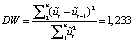 .
.
By setting the boundaries of the critical interval for the DW statistic, we find a positive autocorrelation between random residuals. This may indicate a missing significant explanatory variable in the model (so, the presence of a type 3 error).
Consider the Chow test to check the stability of the estimated model parameters. It is based on the assumption that the random remainder in the linear regression model is normally distributed, homoscedastic, and has no autocorrelation [5, p. 355].
As mentioned, the model under study assumes that there is an artificially created shift due to the transfer of data to another currency. Therefore, divide the sample into two parts – from 2007 to 2010 (inclusive) and from 2011 to 2020. We find two samples composed of the values of the sum of squared residuals ESS’ and ESS’’, as well as the residual sum of squares ESS for the whole sample.
We calculate the random variable of the test statistics and its critical level according to the Fisher distribution Fcr by formulas:
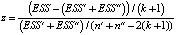 ,
,
Fcr = F.ОБР.ПХ(α; (k + 1);(n' + n'' – 2(k + 1))).
If z < Fcr, then the model parameters are interpreted as the same for the two samples.
The calculated values of z = 3,0893 and Fcr = 2,594 indicate the presence of a structural shift in the analyzed model.
To continue the analysis, we exclude the data for 2007-2010 and re-run the Chow test for a new sample. Between the last quarter of 2014 and the first quarter of 2015, there was a fairly sharp jump in all the model variables, so we will divide the sample again into two parts: from 2011 to 2014 (inclusive) and from 2015 to 2020.
The test results at z = 1,74 и Fcr = 2,74 suggest that the parameters of the estimated model:
 (1)–
(1)–

are constant in the range of changes in the explanatory variables over the entire sample size n = 34.
The optimality of the estimates of the parameters of the model (1) obtained by the least squares method (LSM) can be ensured only if the conditions of the Gauss-Markov theorem are met in it, which are as follows:
1. The columns of the matrix of observed values of the regressors X are linearly independent.
2.  .
.
3. 
4. Cov( , at i ≠ j.
The first condition for the model is met in the course of an earlier analysis of the data for the model.
The second condition can be checked through the R-criterion and the F-test.
Let us introduce the hypothesis 
 .
.
The R-criterion implies finding the coefficient of determination, as well as the adjusted coefficient of determination, using the following formulas:
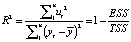
where  – the average value of the endogenous variable
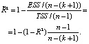
According to the model under study R2 = 0,835, а  , which suggests a very strong explanatory dependency, and the specification is of good quality.
The F-test involves the analysis of a previously defined hypothesis. The following formulas are used:
 ,
,
Fcr = F.ОБР.ПХ(α; k; n – (k + 1)).
If F ≤ Fcr, the hypothesis H0 accepted, and the specification is considered to be of poor quality.
In our case, F = 38,032, Fcr = 2,922, so F ≥ Fcr. Therefore, the hypothesis is rejected, and the specification is recognized as high-quality: the share price of 83,53 % is explained by EBITDA, USD/RUB and inflation.
The second condition of the Gauss-Markov theorem is also met.
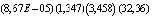
The third condition of the Gauss-Markov theorem is that the variances of the random residuals are equal, and this means that the random residuals are homoscedastic. We will check the compliance with this condition using the Goldfeld-Quandt test, which determines the validity of the hypothesis 
 . To do this, the statistics of the GQ test and its critical level for the F-distribution are calculated using specially prepared data. If GQ < Fcr и GQ-1 < Fcr, then the hypothesis H0 accepted. According to the calculations, GQ = 0,869, GQ–1 = 1,15, Fcr = 3,438, therefore, the hypothesis H0 is accepted, which indicates the homoscedasticity of random residuals.
The fourth condition of the Gauss-Markov theorem indicates that the random residuals in the model are uncorrelated. The analyzed hypothesis – H0: Cov (ui; uj) = 0, at i ≠ j.
The study of this condition by the Darbin-Watson test does not allow the hypothesis H0 to be either accepted or rejected. This is a consequence of removing the structural shift, but since earlier, using more statistics, a positive autocorrelation between random residuals was established for this model, which has certain negative consequences for the LSM estimates of the model parameters, then an adjustment of the model is required. Let’s do this using the Hildreth-Lou and Darbin algorithms. These algorithms are quite similar in their goals-finding the value of the autocorrelation coefficient that minimizes the sum of the squares of the residuals of the transformed model, as well as obtaining more accurate estimates of the parameters to further verify the adequacy of the model.
If the model contains a relationship between adjacent levels of random residuals, its specification takes the form:


where ξt – white noise (a stationary time series with uncorrelated levels that have zero mathematical expectation and the same variance).
Consider the procedure for finding the autocorrelation coefficient using the Hildreth-Lou algorithm.
1. The regression function, which is specified above, is written in a compact form  and the same equation is subtracted from it for the time variable t-1, multiplied by the constant ρ, so
  . The final equation looks like:
 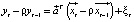 .
.
2. An arbitrary value of ρ is set, with which the estimates of the parameters of the equation from point 1 are found.
3. Using the “Solution Search” tool, we optimize the resulting value of the sum of squares ξt, as an objective function that tends to the minimum when changing a cell with a constant ρ.
4. According to the new parameter estimates, random residuals of the transformed model are found and checked for autocorrelation.
According to the Hildreth-Lu algorithm, the values of ρ = 0,31 were calculated for the sum of squares ξt ESS = 26518,57. Checking the model by the Darbin-Watson test allows us to accept the H0 hypothesis.
According to the Darbin algorithm, the minimum value of the sum of squares ESS = 24937,94 is achieved at ρ = 0.218 and the DW statistics confirm that the random residuals are uncorrelated.
It is evident that the constant ρ is not the same for the two algorithms, therefore, when determining the optimal parameter estimates to check the adequacy of the model must use the algorithm by which the residual sum of squares turned out the least in this case – Durbin algorithm.
Thus, the estimated form of the model, taking into account the autocorrelation of random residuals, is as follows:
 ,
,
 (2)
(2)

We will check the adequacy of the model estimated by the parameters through interval forecasting. To do this, we will see whether the value of the endogenous variable from the control sample is included in the confidence interval or not (if it is, the model is considered adequate). Let’s divide the verification stage into several points:
1. Based on certain values of the regressors from the control sample, we find the point predictive values of the endogenous variable.
2. We calculate the technical error of the forecast  and the standard error of the forecast
  .
.
3. Calculate the critical value tкр = СТЬЮДЕНТ.ОБР.ПХ(α; n – (k + 1)).
4. Find the confidence interval  .
.
The predicted confidence intervals constructed for model (2) for each share price indicator from the control sample (Table 3) at the significance level α = 0,05 are presented in Table 6.
Let’s check whether the obtained interval forecasts cover the actual value of yt from the control sample:
– In September 2013, the share price was 263,71, and it belongs to the confidence interval calculated above;
– In June 2013, the share price was 310,00, and it belongs to the confidence interval calculated above;
– In June 2020, the share price was 361,80, and it does not belong to the confidence interval calculated above;
– In September 2020, the share price was 383,00, and it does not belong to the confidence interval calculated above.
Table 6
Confidence intervals
|
1 |
y- |
168,9535 |
|
y+ |
308,9438 |
|
|
2 |
y- |
211,5723 |
|
y+ |
349,4153 |
|
|
3 |
y- |
171,2433 |
|
y+ |
342,6009 |
|
|
4 |
y- |
215,3058 |
|
y+ |
358,3038 |
Source: Compiled by the author.
It can be seen that the model gave an unconfirmed forecast when using data for 2020, which can be explained by the factor of the pandemic that was not taken into account in the model, which caused serious deviations in the price of the game from the average indicators of previous periods. In the future, a similar econometric analysis may show the presence of a structural shift in 2020. In general, the model is working and adequate with a 95 % probability.
Based on the conducted econometric analysis, a number of conclusions and generalizations can be made.
1. Consideration of the theoretical basis of the study was a necessary tool for this analysis.
2. The specification of the linear multiplier regression model was constructed and the most significant factors were identified.
3. Numerical statistics on endogenous and explanatory variables are collected, training and control samples are defined for the analysis of the constructed model;
4. Various errors were eliminated from the model, a shift was detected, and the model was subsequently corrected. It is shown that the proposed specification is of high quality. It is established that the random residuals in the model are homoscedastic and have a positive autocorrelation. According to the Hildrett-Lu algorithm, it was found that the autocorrelation of the 1st order. Optimal estimates of the model parameters are obtained using the Darbin algorithm.
5. Based on the results of the study as a whole and when checking the predictive properties of the model on the control sample, it was determined that the model is working and adequate. However, it should be assumed that there is a structural shift in 2020, which may give a false assessment of the adequacy of the model under study.
Библиографическая ссылка
Крюкова И.В., Ященко Н.А. ECONOMETRIC FORECAST OF THE SHARE PRICE ON THE EXAMPLE OF PJSC “OIL COMPANY “ROSNEFT” // European Journal of Natural History. 2021. № 2. ;URL: https://world-science.ru/en/article/view?id=34159 (дата обращения: 22.07.2026).
DOI: https://doi.org/10.17513/ejnh.34159