
Scientific journal
European Journal of Natural History
ISSN 2073-4972
ИФ РИНЦ = 0.204
MODELING OF DISTRIBUTION FUNCTIONS IDENTIFYING STUDENTS IN THE PROCESS OF LEARNING

Student knowledge evaluation methods are based on the modeling views on what a student is and how he behaves in the process of gaining knowledge. Two essentially different approaches to the student behavior modeling in the process of gaining knowledge exist (from now on “the process of gaining information” is understood by the phrase “student behavior in the process of gaining knowledge”): first (traditional) approach is based on classical determinacy of student behavior [1]; second approach is based on non-classical determinism (determinism, realized through randomness) [2].
Traditional student model allows to locate student’s position pointwise in the information space, which involves totality of the results of human semantic activity. It is the principle which forms the basis for the point grading method of student knowledge evaluation [3]. Individual knowledge is being evaluated with grades (points), i.e. numbers, and that is pointwise location of student’s position in the information space. Certainly, knowledge evaluation has accuracy (involves error). For the 5-point grading system absolute error is 0,5 point, whereas relative error, divided by the end of scale, is 0,5/5 = 0,1. To reduce relative error one can use 10-point or 100-point scale, which can reduce relative error to 0,05 and 0,005 points accordingly. Such reduction of relative error, of course, increase the accuracy of student knowledge evaluation. However, traditional model is restricted, since it puts out of account random character of student behavior in the process of gaining knowledge.
Probabilistic-statistical student model takes into account random factor in the process of gaining information. According to this model student is identified with a distribution function (probability density) in the information space [4, 5]. This comes from the fact that individual knowledge, being a product of consciousness, is of random character, since the determinism of consciousness is realized through randomness, for it is derived from basically random behavior of psycho-somatic state. In this case non-classical probabilistic statistical method of research is used to describe individual behavior [5]. It should be noted, that traditional student behavior model could be obtained through passing to the limit within the framework of the probabilistic-statistical model. That way, if dispersion of a distribution function, which identify a student, tends to zero, distribution function tends to Dirac delta function (probability density tends to infinity), that defines location of an individual in the information space pointwise. Thus, it is arguable, that probabilistic-statistical model contains traditional student behavior model as its extreme event. The goal of this research is to model distribution functions, which identify students in the process of gaining knowledge.
Materials and research methods
If the point grading system is used for student knowledge evaluation, it is assumed that the measurement range (the maximum scale value) corresponds to the volume of information, that a student can learn during particular course unit or during the whole course. In informatics it is common to measure information in “bits”, whereas in pedagogics - in “points” (grades). One can always set necessary quantitative relation between “bits” and “points”. The grade (points), which student receives as a result of knowledge assessment, is actually an expectation (average value), it defines student’s location pointwise in the information space, putting out of account random character of its knowledge.
To eliminate this shortcoming, one should turn from the point grading method of student’s knowledge assessment to the probabilistic-statistical method, according to which, as it was mentioned earlier, within the information space a student is identified with the distribution function, that accounts for the random character of its knowledge. Such transfer is possible, since the maximum volume of information (the maximum point of a measurement scale), that a student can learn, and an expectation (a grade, which student receive as a result of knowledge assessment) are known for each type of activity. However, knowing it is not enough to graph a “true” distribution function. Hence, let us employ approximation method, which allows to construct so-termed model distribution functions. i.e. functions whose characteristics are close to characteristics of true distribution functions. As a model function we will take level function [6]. In zeroth approximation such function can be presented by one-step (rectangular) function, which corresponds to the uniform distribution of probability density within the scale. But such function can be used to model only symmetric true distribution functions, whose expectation, median and mode are the same and are equal to σ = 0,5σmax, where σ is coordinate. It can’t be used to model asymmetric true distribution functions. In zeroth approximation two-step function can be used as a model distribution function to solve this problem.
Fig. 1 describes qualitatively a true distribution function and corresponding to it two-step model distribution function. To construct a model distribution function, it is essential to find the relation between median σmed, coefficients a and b and expectation <σ>.
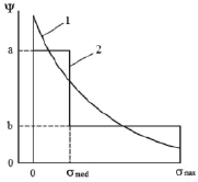
Fig. 1. Distribution function: 1 – true; 2 – model
To determine these coefficients we use an assumption, that probability to find a student within the whole information space is equal to 1 – equation (1), and also use characteristic of a median, which divides distribution function into the two equal parts with respect to the probability to find a student in the information space – equation (2):
 , (1)
, (1)
 . (2)
. (2)
By solving together (1) and (2), we will have:
 and
and  . (3)
. (3)
Expectation will be calculated as an average of the coordinate, and taking account of (1) and (2) it will be as follows:
 . (4)
. (4)
Due to the fact that, when we define student’s knowledge completeness an expectation is being measured, let us determine the link between expectation and median by solving together (3) and (4):
 . (5)
. (5)
From the analysis of (3) and (5) it follows, that if σmed = 0 parameters a, b and <σ> take the following form:
 ,
,  ,
,
 .
.
where δ(σ – 0) is Dirac delta function, equal to zero when σ ≠ 0 and equal to infinity when σ = 0.
Between the limits of zero and maximum scale value integral of delta function is equal to 1. The same is true for σmed = σmax:
 ,
,  ,
,
 .
.
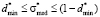
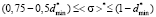
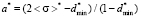
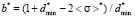
In practice the use of expression (5) is restricted by the measurement error of expectation and median. Suppose that median measurement error is Δσ, since the width of the left step of a model distribution function is the same as a median value (d = σmed), minimum width of the left step of a distribution function is dmin = Δσ, and its maximum width is dmax = (1 – dmin). Hence follow the restrictions on the possible values of median, which can be written as 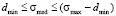 . Then, from this inequation and equation (5) it follows that
 .
.
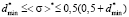
Let us write down this inequation in dimensionless form
 , (6)
, (6)
where  and
and  is a dimensionless relative error and the minimum width of the left step of model distribution function respectively.
According to (5), median-expectation dependence in dimensionless form may be expressed as
 , (7)
, (7)
where  .
.
Expression (7) is true within the range
 . (8)
. (8)
If we use inequation (6) for calculation of distribution functions, coefficients a and b should be dimensionless. For this purpose, we will multiply these coefficients by σmax. Then according to (3) we have
 and
and  , (9)
, (9)
where  and
and  .
.
Within the following range of expectation values
 . (10)
Let us assume, that the width of the left step of distribution function is equal to constant ( ) for all possible values of the expectation. Hence, when expectation changes, only heights of the left and the right steps can change. Such configuration of a model distribution function removes restrictions on the median value. After simple transformations, using equations (3) and (4), for a*, b* and
  we will have
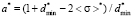 ,
,
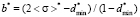 ,
,
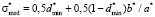 . (11)
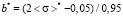
Proceeding similarly within the following range of the values of expectations
 (12)
(12)
and assuming, that the width of the right step of model distribution function remains invariant ( ), we will get
 ,
,
 ,
,
 . (13)
From the joint analysis of (11) and (13) it follows, that the expressions for a* and b* from (11) explicitly agree with the expressions for b* and a* from (13) (crosswise).
Let us visualize the dependence of a*, b* and  on <σ>*. To calculate the required parameters one should know the value of
  , which agrees with the relative error δσ. When evaluation of student’s knowledge is being made with the use of the point grading scales the relative error, divided by the end of scale, usually lies within the limits of 5 % to 10 %. This corresponds to δσ values in the limits of 0,05 to 0,1. Then for definiteness in calculation of specified parameters we should use the relative error equal to δσ = 0,05 (
 ), it significantly simplifies the expressions, which relate these parameters with the expectation within all three tolerance regions of <σ>*. Let us write these relations in a final form.
1st range. By applying  in (10) and (11), we have
 ,
,  ,
,
 ,
,
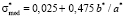 (14)
(14)
2nd range. By applying  in (6)–(9), we have
 ,
,  ,
,
 ,
,
 . (15)
3rd range. By applying  in (12) and (13), we have
 ,
,
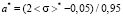 ,
,
 ,
,
 . (16)
Fig. 2 visualizes calculated dependencies of the dimensionless coefficients a*, b* and  from the values of dimensionless expectation.
It is apparent, that coefficients a* and b* are mirror symmetric with respect to the line, that goes through the point with coordinates (0,5; 0) and is parallel to the vertical axe, whereas the median is characterized by rotational symmetry. When the median is rotated by 180 ° with respect to the point with coordinates (0,5; 0,5) it corresponds to itself. Boundaries of the measurement scale answer for such remarkable characteristics of the concerned parameters.
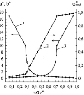
Fig. 2. Dependency of the dimensionless parameters of model distribution function from the values of dimensionless expectation: 1 – parameter a*; 2 – parameter b*; 3 – median σ*med
Research results and discussion
Equations (14) – (16), and also graphics, represented in Fig. 2, could be used to calculate model distribution functions in the dimensionless coordinates. Fig. 3 shows the model distribution functions, which were calculated using equations (14) – (16) for the various values of dimensionless expectation.
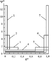
Fig. 3. Distribution functions in the dimensionless coordinates for the various values of dimensionless expectation: 1 – <σ>* = 0,2; 2 – <<σ>* = 0,3; 3 – <σ>* = 0,4; 4 – <σ>* = 0,5; 5 – <σ>* = 0,6; 6 – <σ>* = 0,7; 7 – <σ>* = 0,8
Distribution function  and coordinate
  are represented in the dimensionless form. Model distribution function Ψ*(σ*) is actually a universal function. It has the same form in all point grading measurement systems, it allows to study the behavior aspects of such function and to translate them next onto the model distribution functions in any point grading measurement system, f.e. in 20-point or 100-point grading system. It is achieved by changing the scale factor of the coordinate axes, i.e., multiplying all the numbers on the Y-axis by the maximum value of the selected scale (
 ) and dividing all the numbers on X-axis by the maximum value of the selected scale (
 ).
).
As an example, Fig. 4 shows model distribution functions, identifying students, who have got 3, 4 or 5 points on examination.
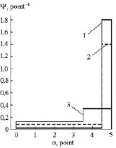
Fig. 4. Distribution function, identifying students, who have got the grades: 1 – 5 points; 2 – 4 points (dashed line); 3 – 3 points
Analysis of data, represented in Fig. 4, shows, that distribution functions 1, 2 and 3 overlays within the range of 4,5 to 5 points. Since the error of 0,5 points, common to the 5-point measurement system, defines the lower limit for the expectation values obtained during the knowledge evaluation, the range of 4,5 to 5 points corresponds to “5” (the result of examination). Then, integration of the distribution function (probability density) over the coordinate in the range of 4,5 to 5 points specifies the probability, that the student will get “5”. In our case the student, who received “5”, received this grade due to the fact, that the probability to learn the educational material amounts to 0,9. Students, who received “4” and “3”, could have got “5” with probability 0,8 and 0,2 respectively.
Conclusions
1. In place of model distribution functions, which approximate empirical distribution functions, identifying students in the process of learning, it is convenient to use two-step functions, that can be calculated on the base of the information about the grades of individuals, which they received after testing using the point grading measurement system.
2. When expectation converges to the boundaries of the measurement scale, probability density of distribution functions tends to infinity. However, probability density could be bounded, if expectation value measurement error is taken into account.
3. Model distribution functions, calculated in the dimensionless coordinates, have the same form in all the point grading measurement systems. This allows to study the behavior aspects of such functions and then to translate them to the model distribution functions in any point grading measurement system.
4. Model distribution functions allow, knowing the grade, that student received in testing, to calculate the probability to get any other grade.
Библиографическая ссылка
Romanov V.P., Shiryaeva N.A. MODELING OF DISTRIBUTION FUNCTIONS IDENTIFYING STUDENTS IN THE PROCESS OF LEARNING // European Journal of Natural History. 2020. № 4. ;URL: https://world-science.ru/en/article/view?id=34111 (дата обращения: 03.06.2026).