
Scientific journal
European Journal of Natural History
ISSN 2073-4972
ИФ РИНЦ = 0.204
VECTOR OPTIMIZATION OF A СОMPLICATED INTELLECTUAL AND MECHANICAL SYSTEMS

Main Definitions
Let us consider a system whose operation is described by a system of equations or whose performance criteria may be directly calculated. We assume that the system depends on r design variables α1,...,αr representing a point α = (α1,...,αr) of an r-dimensional space. In the general case, when designing a system, one has to take into account the design variable constraints, the functional constraints, and the criteria constraints [1].These constraints defines D- the feasible solution set.
Definition 1. A point α0∈D, is called the Pareto optimal point if there exists no point α∈D such that  for all all n = l,...,k, and
  for at least one of n. A set P ⊂ D is called the Pareto optimal set if it consists of Pareto optimal points.
When solving the problem, one has to determine a design variable vector point α0∈P, which is most preferable among the vectors belonging to set P.
The Pareto optimal set plays an important role in vector optimization problems because it can be analyzed more easily than the feasible solution set and because the optimal vector always belongs to the Pareto optimal set, irrespective of the system of preferences used by the expert for comparing vectors belonging to the feasible solution set. Thus, when solving a multicriteria optimization problem, one always has to find the set of Pareto optimal solutions.
The Feasible and Pareto Optimal Sets Approximation
The algorithm discussed in [1] allows simple and efficient identification and selection of feasible points from the design variable space. However, the following question arises: How can one use the algorithm to construct a feasible solution set D with a given accuracy? The latter is constructed by singling out a subset of D that approaches any value of each criterion in region Ф(D) with a predetermined accuracy.
Approximation of Feasible Solution Set
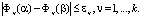
Let εν be an admissible (in the expert’s opinion) error in criterion Фν. By ε we denote the error set {εν}, n = l,...,k. We will say that region Ф(D) is approximated by a finite set Ф(De) with an accuracy up to the set ε, if for any vector α∈D, there can be found a vector β∈De such that
We assume that the functions we will be operating with are continuous and satisfy the Lipschitz condition (L) formulated as follows: For all vectors α and β belonging to the domain of definition of the criterion Фn, there exists a number Lν such that
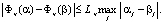
In other words, there exists  such that
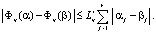
We will say that a function Фν(α) satisfies the special Lipschitz condition (SL) if for all vectors α and β there exist numbers  , j = 1,...,r such that
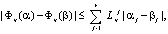
where at least some of the  are different.
Let the Lipschitz constants Lν, be specified, and let N1 be the subset of the points D that are either the Pareto optimal points or lie within the ε-neighborhood of a Pareto optimal point with respect to at least one criterion. In other words, Фν(α0) ≤ Фν(α) ≤ Фν(α0) + εν, where α0∈P, and P is the Pareto optimal set. Also, let N2 = D\N1 and  .
.
Definition 2. A feasible solution set Ф(D) is said to be normally approximated if any point of set N1 is approximated to within an accuracy of ε, and any point of set N2 to within an accuracy of 
Theorem 1. Let the criteria are continuous and satisfies the Lipschitz condition or the special Lipschitz condition. There exists a normal approximation Ф(De) of a feasible solution set Ф(D).
Approximation of Pareto Set
Since the Pareto optimal set is unstable, even slight errors in calculating criteria Фν(α) may lead to a drastic change in the set. This implies that by approximating a feasible solution set with a given accuracy we cannot guarantee an appropriate approximation of the Pareto optimal set. Although the problem has been tackled since the 1950s, a complete solution acceptable for the majority of practical problems is still to be obtained. Nevertheless, promising methods have been proposed for some classes of functions.
Let P be the Pareto optimal set in the design variable space; Ф(P) be its image; and ε be a set of admissible errors. It is desirable to construct a finite Pareto optimal set Ф(Pe) approximating Ф(P) to within an accuracy of ε.
Let Ф(Dε) be the ε-approximation of Ф(D), and Pe be the Pareto optimal subset in De. As has already been mentioned, the complexity of constructing a finite approximation of the Pareto optimal set results from the fact that, in general, in approximating the feasible solution set Ф(D) by a finite set Ф(De) to within an accuracy of ε, one cannot achieve the approximation of Ф(P) with the same accuracy. Such problems are said to be ill-posed in the sense of Tikhonov [2]. Although this notion is routinely used in computational mathematics, let us recall it here.
Let P be a functional in the space X, P:X>Y. We suppose that there exists y* = inf P(x), and Ve(y*) is the neighborhood of the desired solution y*. Let us single out an element x* (or a set of elements) in space X and its d-neighborhood Vd (x*) and call  a solution to the problem of finding the extremum of P if the solution simultaneously satisfies the conditions
  ∈Vδ (x*) and P(
 )∈Vε (y*). If at least one of the conditions is not satisfied for arbitrary values of e and d, then the problem is called ill-posed (in the sense of Tikhonov).
An analogous definition may be formulated for the case when P is an operator mapping space X into space Y. Let us set
X = {Ф(De), Ф(D)}; Y = { Ф(Pe), Ф(P)},
where ε→0, and let P : X>Y be an operator relating any element of X to its Pareto optimal subset. Then in accordance with what was said before, the problem of constructing sets Ф(Dε) and Ф(Pε) belonging simultaneously to the ε-neighborhoods of Ф(D) and Ф(P), respectively, is ill-posed. Of course, in spaces X and Y, the metric or topology, that corresponds to the system of preferences on Ф(D) must be specified [2]. Let us define the Ve-neighborhood of a point Ф(α0)∈Ф(П) as
 .
.
In Theorem 2, a Pareto optimal set Ф(Pε) in which for any point Ф(α0)∈Ф(P) and any of its e-neighborhoods Ve there may be found a point Ф(β)∈Ф(Pε) belonging to Ve is constructed. Conversely, in the e-neighborhood of any point Ф(β)∈Ф(Pε), there must exist a point Ф(α0)∈Ф(P). The set Ф(Pε) is called an approximation possessing property M. Let Ф(Dε), an approximation of Ф(D), have been constructed.
Theorem 2. If the conditions of Theorem 1 are satisfied, then there exists an approximation Ф(Pe) of Pareto set Ф(P) possessing the M-property.
The theorem will be proved by analyzing the neighborhoods of the so-called “suspicious” points from Ф(Dε), that is, the points to whose neighborhoods the true Pareto optimal vectors may belong. If we find new Pareto optimal vectors in the neighborhoods of the “suspicious” points then these vectors may be added to Ф(Pe). Taken together with Ф(Pε), they form the ε-approximation of a Pareto optimal set, [2].
In [2] it is shown that this approach solves the problem of the ill-posedness (in the sense of Tikhonov) of the Pareto optimal set approximation.
Decomposition and Aggregation of Сomplicated Systems
When designing complicated systems, one has to deal with complicated mathematical models. Very often these models have many hundreds of degrees of freedom, are described by high-order sets of equations, and, as has already been mentioned, the calculation of one solution can take an hour or more of computer time. This implies that it is not always possible to solve optimization problems directly (otherwise we would have no problem with large-scale systems). One remedy may be to split (decompose) a complicated system into subsystems that can be easily optimized, and then aggregate the partial optimization results to obtain nearly optimal solutions for the whole system. This will allow a designer to determine the requirements for the subsystems so as to make a machine optimal as a whole and, in this way, justify the proposals for designing different units of the machine.
Construction of Hierarchically Consistent Solutions
To solve this problem we can use an approach associated with considering the whole system as a hierarchical structure .The lower level of this structure comprises subsystems, whereas the higher level is the system as a whole. In many cases, the optimization can be done more simply at the lower level. Therefore, by using the results of the optimization at the lower level and thus reducing the number of competing solutions for the whole system, we can optimize the system in reasonable time. This approach was proposed comparatively recently, and only the first steps have been made in this direction. In particular, this is true for the methods proposed here. Nevertheless, the results obtained can be used to optimize many large-scale systems.
Since the proposed approach is based on the optimization of the whole system through the optimization of its subsystems, we briefly describe the relation between the criteria for the system and subsystems. There are three possibilities for this relation:
1. Some of the criteria of the subsystem can implicitly affect the performance criteria of the system as a whole, and very often, such subsystem criteria are absent from the list of performance criteria of the whole system.
2. Some of the system criteria cannot be calculated at the subsystem level.
3. There are criteria that may be calculated for both the whole system and its sub systems.
The three schemes have the following common features:
1. It is supposed that some of the mathematical models cannot be effectively optimized with respect to the whole criteria vector Ф, because it takes a great deal of computer time to formulate and solve problem of the feasible solutions set determination.. However, the calculation of the values of particular performance criteria Фν needs a reasonable amount of computation.
2. The system is “partitioned” into subsystems. The couplings connecting the subsystems will be called external. To separate out some of the subsystems as autonomous, it is necessary to analyze the interaction of this subsystem with all other subsystems, as well as the external disturbances applied to the subsystem by the environment.
3. There are one or several criteria Фν(α(i)) of the ith subsystem that dominate the corresponding criteria of other subsystems. This means that decreasing (increasing) the values of the criterion Фν(α(i)) by no less than a certain amount εα (for example, Фν(β(i)) > Фν(α(i)) + εα) entails decreasing (increasing) the value of the respective criterion Фν(β) for the whole system, compared with Фν(α). Here, α and β are the design variable vectors of the system, and α(i)) and β(i) are the design variable vectors of the ith subsystem corresponding to the vectors α and β. This condition implies that the system contains one or several subsystems that determine the quality of the system with respect to the νth criterion.
4. It is supposed that the subsystems can be optimized by using the PSI method.
5. Let t be the total time for calculating the values of Фν(α(i)),  and T be the time for calculating the value of Фν(α), where α is the system design variable vector corresponding to all α(i). Then the inequality t << T is assumed to hold.
The idea of optimizing the whole system consists in the following. First, when optimizing each (ith) subsystem, we obtain for this subsystem a pseudo-feasible solution set  , which, as a rule, is somewhat larger than the true feasible solution set. After this, we compile the vectors for the whole system using the respective vectors from the sets
  . On the domain thus obtained, we check whether the criteria and functional constraints of the system are satisfied and, as a result, obtain the feasible solution set D for the whole system. Finally, we search for the optimal solution over the set D.
The main point of this idea is item 3. Let us consider it in more detail. We will say that the pseudo-feasible solution set  for the ith subsystem is dominant if the condition
  entails
  .
.
Theorem 3. In the systems satisfying the aforementioned conditions, there ex-ist subsystems and criteria Фν(α(i)) such that the corresponding pseudo-feasible solution sets  are dominant.
This assertion makes it possible to discard the design-variable vectors α without calculation of the whole system, if the corresponding vector α(i) violates the constraint  . In other words, optimizing the whole system is reduced, to a considerable extent, to the optimization of its subsystems. The schemes given next are based on this idea. These schemes are presented in order of increasing complication. We consider different relationships between the design variables of the system and its subsystems, discuss basic possibilities of simplifying the original model, the ways of determining external disturbances for subsystems, etc.
Let us consider the conditions under which schemes A, B, and C are utilized.
Scheme A
Let us have the mathematical models of subsystems that can be optimized (in a reasonable amount of time). We suppose that each component of the design variable vector,  , of the whole system is a component of at least one subsystem vector α(i) and, on the other hand, that any component of the vector α(i) is a component of the vector α. Therefore, for each of the subsystems, the vector α(i) is uniquely determined by the vector α.
It should be noted that if it is possible to approximate the sets  , the approximation of the feasible solution set for the whole system can be constructed.
However, this procedure is effective only when applied to comparatively simple mechanisms and machines or their units. In more complicated cases, the assumption concerning the relationship between the vectors of design variables α of the whole system and respective vectors α(i) for subsystems are not valid, and we have to use Schemes B and C. Here, situations are possible where the design variable vector of the whole system contains components that are absent from the subsystem level. This can take place, for example, if it is impossible to correctly take into account some external couplings when calculating the subsystem. Therefore, these couplings are usually ignored. Vice versa, among the subsystem design variables, there can be some that weakly (if at all) affect the performance criteria of the system to be optimized. As a rule, these design variables are not included in the list of design variables of the whole system.
Scheme B
Unlike Scheme A, we assume here that the original model is simplified so that it becomes amenable to optimization. Here, external couplings between subsystems are retained, and the simplification is due to either aggregation of solutions for subsystems (this has been mentioned already) or aggregation of internal design variables of the subsystems. Note that, if we succeed in constructing approximations of the sets  ,
,  , we can guarantee that D is nonempty.
Scheme C
We suppose that the system contains a sufficient number of design variables that influence criteria of the subsystem in which they are included and do not affect criteria of other subsystems. By sufficiency we understand that each of the subsystems can be optimized, provided the previous condition is fulfilled. This condition is also necessary because if it turns out that criteria of some subsystem depend on all or almost all of the design variables of the whole system, it will be difficult to optimize this subsystem as the whole system. If this condition is satisfied, we can optimize subsystems in the following two ways.
1. Suppose we can optimize the simplified system for fixed values of the design variables that do not influence the ith subsystem  . In other words, we can optimize the simplified system in a reasonable amount of time, having fixed the system design variables that do not influence criteria of the examined subsystem. External disturbances acting on the subsystem are determined as a result of computations related to the simplified model.
2. If the assumption of item 1 is not valid, the simplified model is not considered. In this case we construct simplified models for each of the subsystems. The simplification of the subsystem model is regarded as acceptable if at least one of the subsystem performance criteria can be calculated with sufficient accuracy and, in addition, the constraint related to this criterion permits us to exclude from consideration a sufficiently large number of design variable vectors α. Having been considered separately, such models of subsystems are not of practical interest. However, provided we have a model of the whole system and the conditions defined above are satisfied, these models facilitate the optimization of the whole system. Note here that external disturbances acting on subsystems are determined not from the model of the whole system, as occurred previously, but from the subsystem models themselves.
Therefore, let all subsystems be optimized, and for each of the subsystems, let the pseudo-feasible solution set  have been obtained according to [1].We define the concatenation operation for the sets
  as follows. Denote by
  the set consisting of vectors
 , such that common (i.e., influencing both subsystems) design variables included in both α(1) and α(2) assume equal values. (If some design variables, such as those describing external couplings, have been omitted when calculating the subsystem, they are added to α(1) and α(2) when constructing vector α). We will denote the result of iterating this operation m times by
  and call the set
  the superstructure over the sets
  . This definition allows us to aggregate different subsystems into the whole system by concatenation of their design variable vectors. Let the sets
  be defined for all
  . The set
  consisting of the design variable vectors of the whole system α such that
  is called the pseudo-feasible solution set for this system. Now let us give the idea of the algorithm for constructing the feasible solution set D. Let us take two subsystems from those obtained after partitioning the system. Suppose there are n common design variables influencing the criteria of both subsystems. We denote these design variables by
  . Let us take an arbitrary vector
  and fix the values of the components
  of this vector. We assume that when probing design variable spaces of the subsystems, we use the points of Pτ nets for each of the subsystems. Then, since the common design variables
  are first in each of the subsystems, they will assume the same values at all points with identical numbers [1]. In
  , we find the vectors α(2) whose first n components assume values equal (to the specified accuracy) to the values of the respective components of the vector α(1). After this, we concatenate the vectors α(2) with the vector α(1). As a result, we obtain the vectors
  . If we find no vector
  that can be concatenated with the vector α(1) the vector α(1) is no longer considered. After performing this operation with all vectors of
  , we obtain the superstructure
  . If there are m subsystems, the process of constructing the superstructure
  is similar. We have only to ensure that the concatenation condition is satisfied. After constructing
  , we calculate the system only at the points of this set. Thus, the original model is calculated repeatedly. However, it is done only on the set
  . If the number of elements in
  is not too large, optimization of the whole system in a reasonable amount of time becomes possible. After introducing constraints
  , we obtain the feasible solution set D. Note that here, as in Scheme B, it is possible that D can turn out to be empty. In this case one should repeat all the described operations until
  . However, D cannot be empty if one succeeds in approximating the sets
  . We denote these approximations by
  .
.
Theorem 4. The set  , being a superstructure over the sets
  , approximates the pseudo-feasible solution set
  of the whole system with a prescribed accuracy.
Corollary. The pseudo-feasible solution set  contains the approximation of the feasible solution set D for the whole system.
Note, that these methods were applied for design of a many- links manipulator and of a car for shock protection. For example, they may be applied to the systemtems described in [3-5].
Conclusion
1. Suggested by author methods of approximation of the feasible solution and Pareto optimal sets are applied to solving the multicriteria optimization problems of complicated systems.
2. The methods of construction of hierarchically consistent solutions are considered.
Библиографическая ссылка
Matusov L.B. VECTOR OPTIMIZATION OF A СОMPLICATED INTELLECTUAL AND MECHANICAL SYSTEMS // European Journal of Natural History. 2019. № 5. ;URL: https://world-science.ru/en/article/view?id=34017 (дата обращения: 26.07.2026).
DOI: https://doi.org/10.17513/ejnh.34017