
Scientific journal
European Journal of Natural History
ISSN 2073-4972
ИФ РИНЦ = 0.204
THE TRANSACTIONAL ASSET PRICING APPROACH (TAPA): APPLICATIONS OF A NEW FRAMEWORK FOR VALUING ILLIQUID INCOME-PRODUCING ASSETS IN THE PROFESSIONAL VALUATION CONTEXT

Ever since A. Marshall brought about the neoclassical synthesis in Economics and I. Fisher developed theories of capital valuation and interest in the early part of XXc., valuation theory has not been static. A particular spurt of activity has been observed in the 1950-1960th when the theory of pricing financial assets has been elaborated starting from works by H. Markovitz W. Sharpe, J. Lintner, as well as Modigliani & Miller. All these works were exploring the brave new world of big financial data, crunching which has suddenly become possible by then newly introduced computer technology, therefore, predicating a valuation theory on distributional statistical concepts of average returns and standard deviations, in the framework of the market efficiency assumption and the homogeneity of market participant expectations, has allowed to frame the standard valuation toolkit of the Modern Portfolio theory (MPT) – which Financial and Business assets valuers (as well as sometimes even Property valuers!) subsequently borrowed for their practical work. After this process of borrowing for the MPT valuation thinking has become assimilated to the actual valuation practice in 1980s and 1990s, the fact that the underlying pricing models perform poorly even in the context of efficient public capital markets, such as in the US, is just relegated to the sidelines of our professional vision (e.g. witness the multitude of ad hoc empirical adjustments, such as premia for company size at odds with the initial underling MPT reasoning, etc., we are forced to put into CAPM to make it work somehow).
But the principle concern for us as Professional valuers is that we usually work with different types of assets than those for which the MPT type of valuation thinking has been originally proposed. The differentiating feature of the assets in this context is their liquidity. Security analysists working with public capital markets –e.g. those people that write buy/hold/sell recommendations for public shares – may find the MPT type valuation theory amenable to their needs in their preoccupation with the issue of long-term fundamental values of liquid (publicly-tradeable) assets. The public markets in which they work may have spot efficiency (i.e. no-arbitrage, the observance of the economic law of one price), but their inter-temporal efficiency is often called into question (i.e. bubbles due to performativity and other “irrationalities”). We, as Professional valuers, whether of businesses or properties, have to admit that we are simply engaged with a different universe of assets. Most asset types covered in the IVSs 2017 –i.e. Property and interests therein, interests in closely-held (non-traded) companies, machinery and equipment, intangibles – are assets with less than perfect liquidity, for which often the current (spot) price is not known (hence, the professional valuers are called to estimate it in the first place!), much less the law of one price is observed. This shows that the use of the MPT pricing models in our Professional valuation (PV) context is an exercise in “by-analogy” thinking fraught with many leaps into the dark: If a valuation of a, say, Romanian village enterprise with some betas and a CAPM model comes to the perusal of a court, the valuer in charge of such a valuation may find hard-pressed to explain himself and give a rationale for the use of the CAPM model in instances where the shares in question are not traded on the public stock exchange, especially if the opposing counsel chips in with a question to the valuer to ask him to explain how the CAPM model of Sharpe and Lintner, implying a single-period forecasting horizon and a homogeneity of market participant expectations, fits into the context of a multi-period DCF analysis deployed, where the expectations of transacting agents on the market with respect to the enterprise cashflows could be different (forming, indeed, the very motive to do a transaction!)?
In my actual courtroom practice of asking such hard questions on the underlying theory of valuation, the valuers blush a lot and default to just saying that it is the current state of professional valuation practice as used. The smarter ones say that the questions are largely justified but that they use the public capital markets pricing mechanism and then introduce a liquidity discount to account for the differences in the pricing approaches as between the unobserved universe of illiquid private assets and the observed universe of liquid public-market related assets. In most instances, such a defense also crumbles when it is found that the valuation report cites some illiquidity discount studies from the American capital market and there are no means to prove that the transference of those discounts to the domestic market context is justified. I have yet to hear a valuer defend himself by alluding to the performativity effect of professional valuations – in that if most valuers follow some accepted valuation practice (doesn’t matter whether a “right” one , or a “wrong” one) the results of valuations will get incorporated into the transaction prices and, overtime, transactions with even illiquid subject assets will converge to mirroring the pricing logic from the public capital market. Alas, this performativity effect would be disconfirmed by the availability of such research as conducted by Robert Slee in his 2004 book on private capital markets [1] and subsequently undertaken empirical Pepperdine University private capital market surveys [2].
Thus, we, as Professional valuers working with less than liquid assets priced on private capital markets (They are also “private” markets in that only a minority of transactions concluded in their context becomes available for research and as a public-domain data in all the essential details. Thus, the notion of a direct and immediate usage of statistical techniques becomes a purely hypothetical one. What is a beta of your apartment?), are essentially left without an uncontroversially applicable valuation theory germane to our environment, instead we are forced to rely on a lot of “by-analogy thinking” borrowed from the procyclicalities-fraught contiguous areas of valuation analyses, such as the valuation of securities on liquid public capital markets.
In the latter area the exclusive reliance on either the market approach or income valuation models based on the static toolset, such as CAPM, create occasionally very strong procyclical negative feedback loops that drive prides of the assets away from their fundamental values.
Is it possible to re-create a valuation theory specifically fit for the context of pricing assets with less than perfect liquidity – without recourse to the pricing models used in the liquid public capital market with which the MPT has richly endowed us? The construction of many such empirical pricing models has been attempted, including the cited attempts by Robert Slee and the Pepperdine University, but so far no comprehensive analytical models have been proposed to re-construct the valuation theory in the required private capital markets context. Because it is really so that unless we develop general analytical models for valuation of illiquid assets, we will be forced to have the ultimate theoretical recourse to the pricing models established –at one, and rather unbridgeable, remove from us-- for the public capital market.
We have been attempting to remedy this situation with the development of the so-called Transactional Asset Pricing Approach (TAPA) over the past decade. In this we proceeded from the meta-assumption that the “unit of analysis” for illiquid asset valuation is a particular transaction (or, sometimes, their set –as in the sales comparison approach), but not the overall general market universe assumed in equilibrium (as in the MPT approach). Thus, we attempt to deduce the analytical model of valuation from the behavior of assumed transacting agents in a particular transaction (and the way they should negotiate their respective economic interests to achieve the balanced transaction), not from the implications of competition between all market agents in the market universe, each possessing the uniformity of expectations about the future. This transaction-based view of asset pricing gave our research program the name “Transactional” in its title.
Our TAPA model has one normative element that incorporates the principle of equity in transaction. This principle is lacking in any formulation for any of the modern pricing models, but in fact has a rich filiation going back through the economic essays of J. Ruskin to Aristotelian “Catallactics’ (the science of exchange) expressed by him in Book V of the Nicomachean Ethics. There were modern-era attempts to reconstruct the investment decision-making and valuation theories based on this principle (for the latest attempt, see e.g [3]). Our formulation for this principle is more dynamic and thus has been given a name of the “inter-temporal principle of transactional equity” (or the fair transaction equilibrium principle). The underlying idea for this principle is that neither of the transacting agents in a priced transaction with an asset should be worse off in consequence of effecting the transaction than their counterparty – by the end of any analysis/forecast period chosen. Analytical decomposition of this principle using the formulas of compound interest with dual rates of return (one for the investment opportunity set of the buyer, and the other – for the investment opportunity set of the seller) allows to provide a general transactional asset pricing model (also featuring dual rates of return with reference to the buyer and the seller). Interested readers are invited to study the analytical derivations in depth by consulting our Paper [4].
The well-known general DCF analysis framework obtains as a specific case of this more general transactional asset pricing model formulation, given the assumption of the equality of discount rates between the buyer and the seller of subject asset. Previously, the DCF analysis framework has been regarded as an artefact resulting from the investor-specific view of asset valuation, as developed in the works of Irving Fisher at the turn of the XX century. Now, TAPA research has made it possible to provide a justification for the DCF analysis on the basis of the inter-temporal principle of transactional equity.
However, there is still one principal – and often overlooked – inconsistency between the explicit multi-period forward-looking orientation of the DCF analysis and the theory of discount rates we use in its context. Most often, we use time-invariant (single-period) discount rates derived from (averaged) historic series of returns (sometimes refracted through the prism of the single-period CAPM or its derivatives). Such a conjunction of the flexible DCF framework, which might well assume the time-variable pattern of performance for the subject asset returns, with the inflexibility of fixed discount rates creates tensions and rigidities in the practical use of the DCF analysis. Indeed, a stand-by court question to a defendant-valuer readily suggests itself here: “In the numerators of the DCF analysis you assume variable returns for your subject asset, what makes you think that the assumed market benchmark of your valuation (Obviously, any valuation under the income approach assumes a certain reference point, or a benchmark. In that sense, income approach valuations are also comparative valuations. The return properties of the valuation benchmark assumed are reflected through the use of a specific discount rate. That is, if the discount rate selected is based on the returns/equity premia of some market index (e.g. S&P 500), then the valuation benchmark assumed in the valuation is the universe of S&P stocks), the performance of which is reflected through the selected discount rate in the DCF denominators, will be characterized by the constancy of returns (the fixed discount rate you use) over the forecast period?” An answer to this question may not always sound convincing, as oftentimes the increased returns for the subject asset in the DCF are projected on the basis of the market surveys or expectations that suggest an improved performance in the market benchmark of valuation (I.e. we may expect an increase in the subject asset returns precisely because the market against which we value such a subject asset is expected to perform better and thus have higher returns over the forecast period selected).
Thus, an important building block for TAPA is its theory of flexible, i.e. time-variant, discount rates. Since the DCF analysis generally assumes a variability in the profile of subject asset returns, it is only fitting that the rates of return for the benchmark adopted in the valuation (i.e. the discount rates) should also be capable of being projected in a time-variable manner (discount rates, that is, not the discount rate). In fairness, modern researchers in the area of Financial Economics have long recognized the issue and are doing something to reform the analytical and valuation practices in this regard. For example, Cochrane’s presidential address to the American Finance Association in 2011 diagnoses the issue right in that most of the changes in asset valuation are due to changes in the market discount rates, not due to changes in the asset’s cash flows. He does a very stellar work in illustrating the matter empirically, but neither he, nor other researchers that subsequently took up his lead in the matter so far succeeded in developing an operational comprehensive analytical model of asset pricing with time-variable discount rates. TAPA, on the other hand, provides such a model of discount rates for the multi-period, multi-asset setting – and in that relies, like CAPM, on the portfolio principle. However, TAPA (unlike CAPM) doesn’t contain any normative assumptions as to how the transacting agents’ portfolios should be formed. This adds to a degree of freedom in actual TAPA-based valuations, because the use of CAPM in any valuation analysis, among other things, implies that the subject investor’s portfolio is composed on the MPT theory principles (i.e. represents a combination of the overall market portfolio with a “risk-free” asset), where it might not actually be the case.
The combination of TAPA discount rate theory with its approach to deriving the DCF framework allows to develop what we call TAPA Basic Pricing Equation (TAPA BPE), which possesses an analytical novelty of tying in the residual value in the DCF analysis (i.e. the terminal value) with the present value of the subject asset being sought (i.e. introducing a circularity element into the DCF framework). Luckily, modern-day spreadsheet capabilities allow for easy solutions to circular equations, thus, we have made TAPA BPE framework easily available for use by Valuers by operationalizing it on an Excel spreadsheet, which anyone can download via this link (https://drive.google.com/open?id = 0B8hVnKfTz9_2aElVTGt2OHNBNTg) and use in their actual property or business valuation practice.
We hold out TAPA as a comprehensive asset pricing framework under the income approach because under certain novel assumptions it reduces to all the known income capitalization formats. For example, TAPA BPE transforms itself into the direct income capitalization format (DIC) (see Table) when we are justified in assuming that the performance of the subject asset (both in terms of its future income and capital value) will exactly mirror the dynamics for the respective valuation benchmark selected. That is, according to TAPA, the Direct income capitalization method is a valid income capitalization technique when the valuer believes that the performance of the subject asset will be exactly the same as that of the market in the context of which it is being valued (over an implicit holding, or forecast, period assumed in the valuation). In a similar vein, TAPA BPE is capable of being reduced to a version of the Gordon formula, with the assumption required to achieve such a reduction being somewhat different from that used in the conventional derivations of the Gordon model. According to TAPA, the derivation of the Gordon formula doesn’t require an assumption of the infinite holding/forecast period, and the formula as presented will be valid in the context of any holding period, provided that the required TAPA assumptions are met: that is, if the subject asset performance, over a forecast period selected, is expected to be identical in terms of its income growth and capital value, but distinct from the performance for the valuation benchmark assumed (That is to say, there is no reason to think that Gordon formula should be used exclusively for valuation of going-concern business entities, the TAPA version of Gordon model is equally applicable to valuation of assets with finite economic lives, provided their income and capital value are assumed to grow or decline at a uniform rate over the selected forecast period). TAPA BPE can also be reduced to Inwood and Hoskold income capitalization formats as shown in the Table [see [4–6]).
By Taylor-expanding the TAPA BPE we also developed what we have called the “quick income capitalization model”, for which there is no precedent in the valuation literature. It is a curio, as we suggest that the full TAPA BPE spreadsheet be used in instances where it is not proving possible to select valuation assumptions, which would reduce the TAPA BPE to specific simple income capitalization formats described above.
Thus, TAPA framework is very productive in explaining in alternative terms when certain income capitalization formats should be used. Additionally, by allowing for time-variant nature of the discount rates, which obtain as TAPA BPE outputs, the TAPA approach can be used as a discount rate forecasting model in its own right—something which seems to be much demanded by the market, given the plethora of empirical surveys on discount rates, such as the Pepperdine University survey already mentioned above. So far, these surveys lack analytical instruments to check their findings for logical consistency. TAPA provides such a tool, as well as serves as a methodology for researching into the fundamental values of capital in the context of cyclical asset valuation.
To summarize our overview of TAPA, TAPA is an explicit model of a comparative valuation under the income approach. The forefront notion of a valuation benchmark is much more fine-tuned in TAPA compared to the traditional DCF applications used by valuers, where it is much more vague (although the discount rate derivation in those also has to allude to some notion of a benchmark, which is often inchoate and exists in the very background of valuation).
Assumptions required to reduce TAPA’ s Basic Pricing Equation to some known income capitalization formats
|
TAPA assumptions: |
Conventional assumptions: |
|||
|
Model |
Subject asset net income over time uo(i) – projected income growth for the subject asset for period i, %; (i = 1..n) where n is a duration of the model forecast period |
Subject asset residual value at the end of the projection period (n-th year) where vo(i) – projected capital value growth for the subject asset for period i,. (i = 1..n) |
Benchmark assumptions where, u(i) – projected income growth for the valuation benchmark for period i, %; v(i) – projected capital value growth for the valuation benchmark for period i, %. (i = 1..n), where n is a duration of the model forecast period |
|
|
Direct income capitalization (DIC)
|
Changes synchronously with the income for the benchmark used uо (i) = u(i) |
Changes synchronously with the benchmark capital values vо (i) = v(i) |
u(i) can be independent from v(i), both can be time-variant (i.e. different for different i) |
Strictly: Perpetual income annuity without growth. In actual practice: a lot of implicit factors also assumed within R, thus confusing market yield with the notion of the cap rate. |
|
Gordon
|
|
|
Constant discount rate: r = R + v, holding when u = v |
Perpetual Income Annuity with the fixed rate of growth |
|
Inwood
|
Constant |
= 0 |
Constant discount rate: r = R + v, holding when u = v |
Assumption of the actual use of the sinking fund, accumulating according to the third money function F(3) |
|
Inwood – extended
|
Constant |
PV•(1 – V) > 0 |
Constant discount rate r = R + v. holding when: u = v |
Assumption of the actual use of the sinking fund, accumulating according to the third money function F(3) |
|
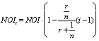
Ring
|
Decreasing:
|
= 0 |
Constant discount rate r = R + v, holding when: u = v |
Assumption for the actual no- interest bearing sinking fund. According to [8]), the assumption of “income foregone”, but no assumption for the actual decline of NOI(i) from the subject asset |


Where:  – Sinking fund factor.
Additionally, TAPA is a multi-period dynamic model of asset values that proceeds from the initial assumption of the bargaining parity between the transacting agents (the TAPA principle of transactional equity). This assumption allows to generalize the DCF approach and recast the traditional DCF framework as a special case of the suggested more general TAPA framework.
Could it be that TAPA is a step in a right direction towards a suitable unified foundational theory for the Professional valuation specialisms, including business and property valuation? Since the departure point for TAPA is the dynamic modelling of a transaction, and not of a general market universe, TAPA can be regarded as an analytical valuation theory for the valuation of assets with less than perfect liquidity and having regard to the explicit cyclical nature of the assets (see [7]). Are not such assets – whether in business, property or intangibles valuation specialisms – the basic subject matter of the Professional valuation? At least it can be said that where a valuation explicitly requires the adoption of a transactional-based view, as in instances of estimating Equitable (as per IVS 2017 definition), or Fair (as per EVS 2016 definition) Value, TAPA provides the readily available methodological approach for valuing income-producing assets, which can be considered and eventually applied by valuers.
The Paper has been prepared under the sponsorship of a grant from the Russian Foundation for Science (RNF) (grant № 18-18-00488).
Библиографическая ссылка
Michaletz V.B., Artemenkov A.I., Medvedeva O.E. THE TRANSACTIONAL ASSET PRICING APPROACH (TAPA): APPLICATIONS OF A NEW FRAMEWORK FOR VALUING ILLIQUID INCOME-PRODUCING ASSETS IN THE PROFESSIONAL VALUATION CONTEXT // European Journal of Natural History. 2019. № 5. ;URL: https://world-science.ru/en/article/view?id=34009 (дата обращения: 02.07.2026).