
Scientific journal
European Journal of Natural History
ISSN 2073-4972
ИФ РИНЦ = 0.204
CONSTRUCTION AND THE ANALYSIS OF MATHEMATICAL MODELS OF EDUCATION

The study of constructed models plays important role together with the construction of mathematical model. One of the methods of analyzing the models that use systems of differential equations is the analysis of the solution stability. There are several methods of the examination of the stability of the differential equations solutions. The stability of solutions in terms of Lyapunov has been used in this article. The stability in terms of Lyapunov implies the study of the endless time interval. The question of asymptotic stability is being analised in the article since we are interested not only in final interval during higher education, but also saving the residual knowledge.
Let us divide a set of students into three groups. The first one consists of the students that are strong at studies, the second one - of those that are average at it, and the third group consists of weak students. This distribution is conditional, it doesn´t reflect the degree of natural gifts, internal preparation, diligence, motivation. However the study of even such simple model allows us to obtain interesting qualitative material.
In the first model let us assume that the knowledge is distributed equally within all three groups.
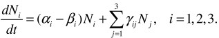
Let us designate the level of knowledge within students in group i as Ni (t), i = 1,2,3, and the operating influence on group i as Ui (t). The operating influence can be persistent, discrete (control measures), or of combined type. Let us introduce coefficients: ![]() - the coefficient of knowledge within group i, βi - the coefficient of the forgetting of school material, δi - the coefficient of the controllability of group i, εi- the coefficient of the controllability of group i depending on the tutor´s qualification level, γij- the coefficient of the impact of group i upon group j. As a result we have simple model:
- the coefficient of knowledge within group i, βi - the coefficient of the forgetting of school material, δi - the coefficient of the controllability of group i, εi- the coefficient of the controllability of group i depending on the tutor´s qualification level, γij- the coefficient of the impact of group i upon group j. As a result we have simple model:
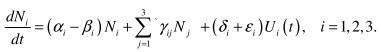 (1)
(1)
As initial conditions we take initiall preparation of group. ![]() implies the summing on i ≠ j
implies the summing on i ≠ j
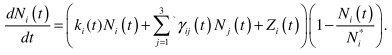
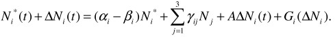
Let us introduce some accurate definitions into the model (1). Coefficients ![]() are dependent on time. We will take the effect of satiation into consideration, according to which the amount of knowledge within every group cannot exceed some utmost value Ni*, that is special for every group. Finally, for every group there is a limit of operating influence that we will designate as
are dependent on time. We will take the effect of satiation into consideration, according to which the amount of knowledge within every group cannot exceed some utmost value Ni*, that is special for every group. Finally, for every group there is a limit of operating influence that we will designate as ![]() . Considering this remarks, the model will take on form:
. Considering this remarks, the model will take on form:
 (2)
(2)
The initial conditions are the same as for model (1).
In models (1) and (2) it was supposed that the knowledge had been distributed equally within the group. Let us renounce this supposition, assuming that the distribution of knowledge is going on according to parameter r. For the strongest student r = 0. Then the model will take on form:

![]() (3)
(3)
ηi (r, t) here is the coefficient of knowledge transmission in group i. The level of initial preparation is taken as initial values in model (3).
Let us study the dynamics of the educational processes, that has been obtained in numerical realization of models (1)-(3).
In simple model (1) Ni (t) (i = 1,2,3) shows the level of knowledge within the students of group i at the temporal moment t. If we define coefficients αi - βi = ki , then the model will take on form:
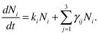
This system can be also put down as:
![]()
The solution of this system should be searched in form:
![]()
where λi are characteristics of the number of matrix A, pij are coordinates of inherent vectors.
Fundamental system of the solutions takes on form:
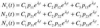
The permanent integrations of C1 , C2 , C3 can be found from the condition Ni (0) = Ni0 - the initial amount of knowledge in the beginning of education. As we adjust the coefficient of operating influence δi, we will obtain different images of the system outgoing.
Let us study the dynamics of the educational process considering satiation. This phenomenon is described in work [1]. Let us introduce one more definition:

Model (2) will take on form:
In general view the system looks that way:
![]()
The solution is being searched in the following form:
![]()
where t is independent variable (time).
Comparing the results of the realization of models (1) and (2) we can notice that in the first case the amount of knowledge grows unreservedly and within the second model the process of satiation takes place and the amount of knowledge doesn´t exceed definite limit. Such picture is more realistic so it is reasonable to use model (2).
The research of the stability of the solutions of various models comes to study of the system of non-linear differential equations [3]. The analysis of the stability of non-linear problems comes to study of the stability of linear equation solutions.
Let the stability of stationary solution of the system of non-linear differential equations of type (1) ![]() . Vector
. Vector ![]() is called the point of balance or the special point if the tutorial influence on the educational process is not considered. The equations system takes on form:
is called the point of balance or the special point if the tutorial influence on the educational process is not considered. The equations system takes on form:
 (4)
(4)
Let us study the little deviation from the special point:
![]()
As we decompose this function into the lines of Taylor, we have:
Jacobian matrix A, function G are formed by non-linear to ΔN terms of decomposition. We use the first method of the study of stability according to Lyapunov. Matrix A does not have inherent values with zero valid parts and multiple to inherent values, that is why while studying the stability if solution ![]() the rest of line
the rest of line ![]() can be set aside. In work by I.V. Boykov [5] the theorem about the stability of systems of differential equations is proved is the condition is met:
can be set aside. In work by I.V. Boykov [5] the theorem about the stability of systems of differential equations is proved is the condition is met:
![]()
where is logarithmic norm. The solution is stable, if the grubs of characteristic equation lie in left half-plane. As we move to new basis we come to linear system of differential equations. Re λk <0. The valid part of inherent values is less than zero and the state of balance will be stable.
References:
- Kapitsa S.P., Kudryumov S.P., Malinetskiy G.G. Synergy and the prognosis of future. Moscow, Editorial URSS, 2003. 288 p.
- Dobrinina N.F. The problems of the stability of the dynamic models of education solutions. Analytic and numeral methods of scientific and social problems modeling. The collection of articles of the 4th International scientific-technical conference. Penza, Privolzhskiy house of knowledge, 2009. P. 274-279.
- Boykov I.V. The stability of the solutions of differential equations. Penza, Penza State University Publishing, 2008. 244 p.
Библиографическая ссылка
Dobrynina N. CONSTRUCTION AND THE ANALYSIS OF MATHEMATICAL MODELS OF EDUCATION // European Journal of Natural History. 2010. № 3. ;URL: https://world-science.ru/en/article/view?id=21032 (дата обращения: 20.05.2026).