Scientific journal

European Journal of Natural History

ISSN 2073-4972

ИФ РИНЦ = 0,301

The Main Definitions

Let us consider a artificial intelligence or mechanical system, whose opera

tion is described by a system of equations or whose performance criteria may be directly calculated. We assume that the system depends on r design variables α α1,...,αr representing a point α = (α1,...,αr) of an r-dimensional space . In the general case, one has to take into account the design variable constraints, the functional constraints, and the criteria constraints [1].There also exist particular performance criteria, such as productivity, materials consumption, efficiency and so on. It is desired that, with other things being equal, these criteria, denoted by Ф_v(α), n = l,...,k, would have the extreme values. For simplicity, we assume that Ф_v(α), are to be minimized.

In order to avoid situations in which the expert regards the values of some criteria as unacceptable, we introduce the criteria constraints

n = l,...,k, (1)

where is the worst value of criterion Ф_v(α) to which the expert may agree.

The criteria constraints differ from the functional constraints in that the former are determined when solving a problem and, as a rule, are repeatedly revised. Hence, reasonable values of cannot be chosen before solving the problem.

The design variable constraints, the functional constraints and the criteria constraints define the feasible solution set D [1].

Let us formulate one of the basic problems of multicriteria optimization.

Definition 1. A point α⁰∈D, is called the Pareto optimal point if there exists no point α∈D such that for all n = l,...,k, and for at least one .

A set P⊂D is called the Pareto optimal set if it consists of Pareto optimal points. When solving the problem, one has to determine a design variable vector point α⁰∈P, which is most preferable among the vectors belonging to set P.

The Pareto optimal set plays an important role in vector optimization problems because it can be analyzed more easily than the feasible solution set and because the optimal vector always belongs to the Pareto optimal set, irrespective of the system of preferences used by the expert for comparing vectors belonging to the feasible solution set.

Construction of the Feasible Solution Set With Prescribed Accuracy The Estimation of the Convergence Rate

The algorithm discussed in [1] allows simple and efficient identification and selection of feasible points from the design variable space. However, the following question arises: How can one use the algorithm to construct a feasible solution set D with a given accuracy? The latter is constructed by singling out a subset of D that approaches any value of each criterion in region Ф(D) with a predetermined accuracy. Let ε_v be an admissible (in the expert’s opinion) error in criterion Фn. By ε we denote the error set {ε_v}, n = l,...,k. We will say that region Ф(D) is approximated by a finite set Ф(De) with an accuracy up to the set ε, if for any vector α∈D, there can be found a vector β∈D_e such that

We assume that the functions we shall be operating with are continuous and satisfy the Lipschitz condition (L) formulated as follows: For all vectors α and β belonging to the domain of definition of the criterion Ф_v(α), there exists a number L_v such that

In other words, there exists such that

We will say that a function Ф_n(α) satisfies the special Lipschitz condition (SL) if for all vectors α and β there exist numbers , j = 1,...,r such that

,

where at least some of the are different.

Let [Lv] (or []) be a dyadic rational number exceeding Lv (or ) and sufficiently close to the latter, and let [ε_v] be the maximum dyadic rational number that is less than or equal to ε_v and whose numerator is the same as that of [Lv] (or []). A dyadic number is a number of the form p/2m, where p and m are natural numbers.

Theorem 1. If criteria Ф_v(α) are continuous and satisfy either the Lipschitz condition or the special Lipschitz condition, then to approximate Ф(D) to within an accuracy of ε it is sufficient to have

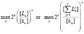
points of the P_τ net [2]. (For details on τ and the Pτ net, see [1].)

The number of points needed to calculate the performance criteria in this estimate may be so large that the speed of computers may prove to be inadequate. This difficulty may be overcome by developing “fast” algorithms dealing not with an entire class of functions but instead taking into account the features of the functions of each concrete problem. Let the Lipschitz constants Lv , be specified, and let N1 be the subset of the points of D that are either the Pareto optimal points or lie within the ε-neighborhood of a Pareto optimal point with respect to at least one criterion. In other words, Фν(α⁰) ≤ Фν(α) ≤ Фν(α⁰) + ε_ν, where α⁰∈P, and P is the Pareto optimal set. Also, let N2 = D\N1 and .

Definition 2. A feasible solution set Ф(D) is said to be normally approximated if any point of set N1 is approximated to within an accuracy of ε, and any point of set N2 to within an accuracy of

In next theorem the algorithm of approximation is given [3].

Theorem 2. If criteria Ф_v(α) are continuous and satisfy either the Lipschitz condition or the special Lipschitz condition, then there exists a normal approximation Ф(De) of a feasible solution set Ф(D).

Multicriteria Simulation

In this section we will describe applying above mention results to solving a multicriteria identification problems of artificial intelligence, medical engineering and mechanical systems. As a rule these applied identification problems have been treated as single-criterion problems. In the majority of conventional problems, the system is tacitly assumed to be in full agreement with its mathematical model. However, for complex engineering systems we generally cannot assert a sufficient correspondence between the model and the object. This does not permit us to use a single criterion to evaluate the adequacy. In multicriteria identification problems there is no necessity of artificially introducing a single criterion to the detriment of the physical essence of the problem.

Parametric identification is reduced to finding numerical values of the equation coefficients, based on the realization of the input and output processes. In doing so, frequency responses, transfer functions, and unit step functions are often used. A number of problems require preliminary experimental determination of the basic characteristics of a system (e.g., the frequencies, shapes, and decrements of natural oscillations). In identification problems we will deal with particular adequacy (proximity) criteria. By adequacy (proximity) criteria we mean the discrepancies between the experimental and computed data, the latter being determined on the basis of the mathematical model. For example, when identifying the parameters of the dynamical model of an automobile it is necessary to take into account such important indices (particular criteria) as vibration accelerations at all characteristic points of the driver’s seat, driver’s cab, frame, and engine; vertical dynamical reactions at contact areas between the wheels and the road; relative (with respect to the frame) displacements of the cab, wheels, engine, etc.

In all basic units of the structure under study we experimentally measure the values of the characteristic quantities of interest (e.g., displacements, velocities, accelerations, etc.). At the same time we calculate the corresponding quantities by using the mathematical model. As a result, particular adequacy (proximity) criteria are formed as functions of the difference between the experimental and computed data. Thus we arrive at a multicriteria problem. The multicriteria consideration makes it possible to extend the application area of the identification theory substantially.

Defining the Feasible Solution Set and the Adequate Vectors

We denote by the indices (criteria) resulting from the analysis of the mathematical model that describes a physical system, where α = (α1,...,α_r) is the vector of the parameters of the model. Let be the experimental value of the criterion measured directly on the prototype. The experiment is assumed to be sufficiently accurate and complete. Suppose there exists a mathematical model or a hierarchical set of models describing the system behavior. Let , where is a particular adequacy (closeness, proximity) criterion[4]. This criterion, as has already been mentioned, is a function of the difference (error) . Very often it is given by or . If the experimental values are measured with considerable error, then the quantity can be treated as a random variable. If this random variable is normally distributed, the corresponding adequacy criterion is expressed by , where denotes the mathematical expectation of the random variable . For other distribution functions, more complicated methods of estimation are used, for example, the maximum likelihood method.

We formulate the following problem by comparing the experimental and calculation data, determining to what extent the model corresponds to the physical system, and finding the variables of the model. In other words, it is necessary to find the vectors αⁱ satisfying the design variable constraints, the functional constraints, and the next criteria constraints

(2)

These constraints define the feasible solution set D_α. Here, are criteria constraints that are determined in the dialogue between the researcher and a computer. To a considerable extent, these constraints depend on the accuracy of the experiment and the physical sense of the criteria .The formulation and solution of the identification problem are based on the parameter space investigation method. We specify the values and find vectors meeting the design variable constraints, the functional constraints, and the criteria constraints. The vectors belonging to the feasible solution set D_α will be called adequate vectors. The restoration of the parameters of a specific model is the main purpose and essence of multicriteria parametric identification. Having performed this procedure for all structures (mathematical models), we thus carry out multicriteria structural identification.

The vectors that belong to the set of adequate vectors and have been chosen by using a special decision making rule will be called identified vectors.

The role of the decision making rule is often played by nonformal analysis of the set of adequate vectors. If this analysis separates several equally acceptable vectors , the solution of the identification problem is nonunique.

The identified vectors form the identification domain . Sometimes, by carrying out additional physical experiments, revising constraints etc., one can reduce the domain Did and even achieve the result that this domain contains only one vector. Unfortunately, this is far from usual. Nonunique restoration of variables is a recompense for the discrepancy between the physical object and its mathematical model, incompleteness of physical experiments, etc.

If a mathematical model is sufficiently good (i.e., it correctly describes the behavior of the physical system), then multicriteria parametric identification leads to a nonempty set D_α. The most important factors that can lead to an empty D_α are imperfection of the mathematical model and lack of information about the domain in which the desired solutions should be searched for.

The search for the set D_α is very important, even in the case where the results are not promising. It enables the researcher to judge the mathematical model objectively (not only intuitively), to analyze its advantages and drawbacks on the basis of all proximity criteria.

The Search For Identified Solutions With Prescribed Accuracy

Let characterize the desired accuracy of the correspondence between the physical system and its mathematical model with respect to the criterion (i.e., the inequality must hold). Then the values of all criteria restoring the experimental characteristics with a prescribed accuracy can be found through the approximation of the adequacy criteria range.

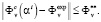
In multicriteria identification, we are interested not only in values of adequacy criteria, but also in values of variables. For example, let α and β be vectors giving “good” values to adequacy criteria, i.e., , while at the same time the vectors α and β are significantly different. In this case, if there is no additional information available for making the choice between the vectors α and β, we can regard as being equally adequate to the physical experiment. However, the researcher must keep in mind all vectors corresponding to good values of adequacy criteria. This is explained by the following considerations. In practice, it is usually impossible to formalize all requirements imposed on a physical or engineering system. If we take into account only one of two vectors corresponding to approximately the same values of adequacy criteria, we may possibly lose the better vector with respect to nonformalized criteria. Suppose we have succeeded in meeting all the demands of the system. In this case, we should consider all the aforementioned vectors when working with the mathematical model after completing the identification. Suppose we are to optimize the parameters of the model with respect to some criteria. If we have eliminated one of two equally adequate vectors, the dropped vector can turn out to be the preferred one with regard to the performance criteria. Taking into account these considerations, we can modify the definition of the solution of the multicriteria identification problem.

We denote by V_εФ(Р) an ε-neighborhood of the Pareto optimal set Ф(Р) in the space of adequacy criteria. It is reasonable to define the solution of the multicriteria identification problem as a set W_ε of all variable vectors α belonging to the feasible solution set D_α and satisfying the inclusion

As a result of nonformal analysis of the set W_ε, the researcher can choose the most preferred vectors.

Let us show how one can solve the problem by using the parameter space investigation method.

The solution algorithm is based not only on the approximation of the criteria space, but also on the approximation of the variable space. Let , and δ_{k + j} be the admissible error for the variable α_j, where k is the number of adequacy criteria. By using the algorithm of Theorem 2, let us construct the approximation of the set D_α to the accuracy , and the approximation of its image Ф(D_α), to the accuracy . The fact that we have declared the variables α_j as criteria Ф_{k + j}, enables us to approximate Ф(D_α) and D_α simultaneously. In this case, the set V_εФ(Р) can be approximated to the accuracy ε, and any vector of D_α can be determined to the accuracy δ Using the approximations of D_α, and Ф(D_α) we can find the set Wε, and thus obtain the solution of the multicriteria identification problem.

Let us call the set Wε the set of ε-adequate vectors. The vectors α_id that belong to the set of ε-adequate vectors and are determined with the help of a decision-making rule will be called identified vectors. The set D_id of all identified vectors is called the identification set.

The work is submitted to the International Scientific Conference “Computer simulation in science and technology”, UAE (Dubai), 4-10 March 2018, came to the editorial office оn 10.10.2018.